
2. Activation functions
Each layer computes a pre-activation \(z^{[l]} = W^{[l]} a^{[l-1]} + b^{[l]}\) and then an activation \(a^{[l]} = g^{[l]}(z^{[l]})\). The choice of the nonlinearity \(g^{[l]}\) is what makes depth worthwhile. This lesson explains why a nonlinear \(g\) is required, surveys the sigmoid, tanh, and ReLU families, introduces the softmax used at the output, and gives practical guidance on which activation to pick.
2.1 Why nonlinearity is required
Suppose every activation were the identity, \(g^{[l]}(z) = z\). Then each layer is just \(a^{[l]} = W^{[l]} a^{[l-1]} + b^{[l]}\), and composing two of them gives \(W^{[2]}(W^{[1]} x + b^{[1]}) + b^{[2]} = (W^{[2]} W^{[1]}) x + (W^{[2]} b^{[1]} + b^{[2]})\). That is again of the form \(W x + b\). By induction the whole \(L\)-layer network reduces to a single affine map:
\[\boxed{ g^{[l]} = \text{identity} \;\Rightarrow\; \hat{y} = W' x + b' }\]with \(W' = W^{[L]} \cdots W^{[1]}\) and \(b'\) the accumulated bias. No matter how many linear layers are stacked, the model can only fit a linear function, so the extra depth buys nothing. A nonlinear \(g\) between layers is exactly what breaks this collapse and lets the network represent curved decision boundaries and nonlinear regressions.
Remark: the bias is kept explicit here as \(b^{[l]}\), unlike the Machine Learning course where the intercept was folded into \(w^T x\) via the augmented input \(x_0 = 1\). In this Deep Learning course each layer has its own weight matrix \(W^{[l]}\) and its own bias vector \(b^{[l]}\).
2.2 Sigmoid and tanh
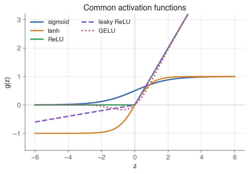
Common activation functions: the bounded sigmoid and tanh saturate in their tails, while ReLU and its variants stay linear for positive inputs.
2.2.1 Sigmoid
The sigmoid squashes any real pre-activation into the open interval \((0, 1)\):
\[\boxed{ \sigma(z) = \frac{1}{1 + e^{-z}} \in (0, 1) }\]Its derivative has the convenient closed form below, which reuses the forward value \(\sigma(z)\) already computed:
\[\boxed{ \sigma'(z) = \sigma(z)\left(1 - \sigma(z)\right) }\]2.2.2 Tanh
The hyperbolic tangent is a rescaled sigmoid centred at zero, with output in \((-1, 1)\). Its derivative is likewise expressible from the forward value:
\[\boxed{ \tanh'(z) = 1 - \tanh(z)^2 }\]Remark: \(\tanh\) is zero-centred while \(\sigma\) is not, so \(\tanh\) often trains a little better as a hidden activation. The two are related by \(\tanh(z) = 2\sigma(2z) - 1\).
2.2.3 Saturation
Both curves flatten in their tails. For large \(|z|\) the output is close to a constant (\(0\) or \(1\) for \(\sigma\), \(\pm 1\) for \(\tanh\)), so the derivative is close to zero: \(\sigma'(z) \to 0\) and \(\tanh'(z) \to 0\). A unit sitting in that flat region is said to saturate, and it passes almost no gradient backward. When many such factors multiply through a deep stack the gradient shrinks toward zero: the vanishing gradient, made precise in the next section.
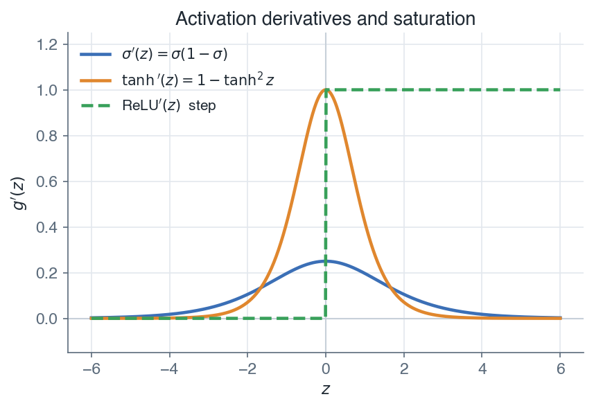
Activation derivatives: sigmoid and tanh gradients vanish in the tails, whereas the ReLU gradient is 1 wherever the unit is active.
2.3 The vanishing gradient
Saturation is not a cosmetic flaw, it decides whether a deep stack can train at all. Backpropagation multiplies the error by the local slope \(g'(z^{[l]})\) at every layer it crosses, so the gradient reaching layer 1 contains one such factor per layer. With sigmoid activations those factors are small by construction: section 2.2.1 gave \(\sigma'(z) = \sigma(z)(1 - \sigma(z))\), and that product never exceeds
\[\boxed{ \sigma'(z) = \sigma(z)\left(1 - \sigma(z)\right) \le \tfrac{1}{4} }\]The result is the vanishing gradient: the layers near the output learn, the layers near the input receive almost nothing and barely move. Deep sigmoid networks stall, and the fix is not a better optimizer, it is a better activation, the ReLU of the next section.
Proof: the gradient shrinks geometrically with depth
Step 1: the sigmoid's slope never exceeds \(1/4\). Write \(s = \sigma(z) \in (0, 1)\). The product \(s(1 - s)\) is a downward parabola in \(s\), largest at \(s = \tfrac{1}{2}\) where it equals \(\tfrac{1}{4}\). So the bound holds, with equality only at \(z = 0\), and saturation makes it far worse: a unit sitting at \(\sigma(2) \approx 0.88\) already has slope \(0.88 \cdot 0.12 \approx 0.10\).
Step 2: backpropagation multiplies those slopes. Take the simplest deep network, a chain of \(L\) layers with one unit each, so every quantity is a scalar. Each layer crossed contributes the factor \(\partial z^{[l]} / \partial z^{[l-1]} = w^{[l]}\, \sigma'(z^{[l-1]})\):
\[\frac{\partial L}{\partial z^{[1]}} = \frac{\partial L}{\partial z^{[L]}} \prod_{l=2}^{L} w^{[l]}\, \sigma'(z^{[l-1]})\]With weights of typical size \(|w^{[l]}| \le 1\), every factor is at most \(\tfrac{1}{4}\) in absolute value, so
\[\boxed{ \left|\frac{\partial L}{\partial z^{[1]}}\right| \le \left(\tfrac{1}{4}\right)^{L-1} \left|\frac{\partial L}{\partial z^{[L]}}\right| }\]
Ten layers already shrink the gradient by about \(10^{-6}\). \(\blacksquare\)
Weights much larger than \(1\) only trade the problem for its mirror image, the exploding gradient. Training deep networks picks the weight scale so this product stays near \(1\).
2.4 The ReLU family
The rectified linear unit keeps the positive part of its input and zeroes the rest:
\[\boxed{ \text{ReLU}(z) = \max(0, z) }\]Its derivative is \(1\) for \(z > 0\) and \(0\) for \(z < 0\) (undefined at \(z = 0\), taken to be \(0\) or \(1\) by convention). ReLU does not saturate on the positive side, so it keeps a healthy gradient flowing there, which is a large part of why it became the default hidden activation. The cost is the dead-unit problem: if a unit's pre-activation is always negative across the data, its gradient is always zero and it stops learning entirely. The variants below trade a little simplicity to soften that failure or to smooth the kink at the origin.
| name | formula | derivative | dies / saturates? |
|---|---|---|---|
| ReLU | \(\max(0, z)\) | \(1\) if \(z>0\) else \(0\) | can die (zero gradient for \(z<0\)) |
| Leaky ReLU | \(\max(\alpha z, z)\), \(\alpha \approx 0.01\) | \(1\) if \(z>0\) else \(\alpha\) | rarely dies (small negative slope) |
| PReLU | \(\max(\alpha z, z)\), \(\alpha\) learned | \(1\) if \(z>0\) else \(\alpha\) | rarely dies (\(\alpha\) trained per channel) |
| ELU | \(z\) if \(z>0\) else \(\alpha(e^z - 1)\) | \(1\) if \(z>0\) else \(\alpha e^z\) | saturates gently for \(z\to-\infty\) |
| GELU | \(z\,\Phi(z)\), \(\Phi\) the normal CDF | smooth, near \(1\) for large \(z\) | smooth, no hard death |
Remark: leaky ReLU and PReLU add a small slope \(\alpha\) on the negative side so a unit is never fully switched off. GELU weights the input by the probability \(\Phi(z)\) that a standard normal is below \(z\), giving a smooth curve that behaves like ReLU for large \(|z|\). It is the standard choice inside Transformers.
2.5 Softmax for multiclass outputs
For a classification with \(K\) classes the final layer outputs a vector \(z \in \mathbb{R}^K\) of scores, and the softmax turns it into a probability distribution over the classes:
\[\boxed{ \text{softmax}(z)_k = \frac{e^{z_k}}{\sum_{j=1}^{K} e^{z_j}} }\]Each component lies in \((0, 1)\) and the components sum to \(1\), so \(\text{softmax}(z)_k\) reads as the predicted probability of class \(k\). The largest score becomes the most likely class.
Remark: softmax belongs at the output layer, not in a hidden layer. It couples every unit through the shared denominator (a normalization across the whole vector), which is exactly what a probability output needs but is not a useful per-unit hidden nonlinearity. For a single output (\(K = 1\) vs its complement) softmax reduces to the sigmoid. The pairing of softmax with its loss was settled in section 6.3 of Multilayer neural networks.
2.6 Choosing an activation
A useful default: use ReLU or GELU in the hidden layers, and choose the output activation from the task. The diagram and table below summarize the decision.
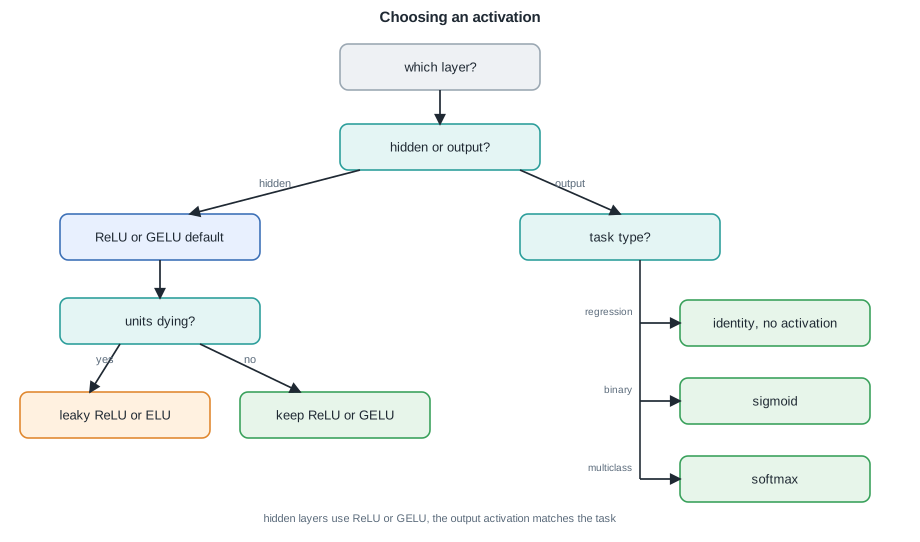
Choosing an activation: ReLU or GELU for hidden layers, and an output activation matched to the task.
| layer / task | recommended activation | reason |
|---|---|---|
| hidden (default) | ReLU or GELU | no positive-side saturation, cheap, trains fast |
| hidden (dead units) | leaky ReLU or ELU | keeps a nonzero gradient for \(z < 0\) |
| output, regression | identity (none) | prediction is an unbounded real value |
| output, binary | sigmoid | maps score to a probability in \((0, 1)\) |
| output, multiclass | softmax | maps scores to a distribution over classes |
Remark: sigmoid and tanh are now rarely used as hidden activations in deep feed-forward networks precisely because of the saturation in Section 3.2.3. They survive at the output (sigmoid) and inside gated recurrent units, where their bounded range is the point.
With the per-layer nonlinearities fixed, the next lesson turns the gradients into updates: the optimizers that make deep training practical.
Next: Optimization · Course overview